sc3D Viewer

A plugin to visualise 3D spatial single cell omics

---

This napari plugin was generated with Cookiecutter using @napari's cookiecutter-napari-plugin template.

Test and atlas datasets¶

Because the datasets representing the mouse embryo at stages E8.5 and E9.0 are rather large, it is not possible to host them on GitHub. They are instead hosted on figshare at the following links:

• E8.5 replicate 1
• E8.5 replicate 2
• E9.0 replicate 1

Once downloaded, one can open them in the viewer as explained below (note that the files for the tissue names are stored in the json file there: napari-sc3D-viewer/test_data/corresptissues.json). It can be downloaded by right-clicking on the following link and then clicking on "Save link as".

Installation¶

---

Disclaimer: While we tried to make the installation and usage as easy as possible, please keep in mind that napari-sc3d-viewer is still under development, it has been and is being developed by a single person. We will be happy to answer any question and help in any way.

---

There are many ways to install our viewer, but the global idea is that it works in two steps:

• first installing napari
• then installing the napari-sc3d-viewer plugin.

Installing napari and the napari-sc3d-viewer plugin can be done either through command line or using an interface.

If you have decided to use command line, as napari developers do, we strongly recommend to install the viewer in an environement such as a conda environment conda for example:

conda create -n sc3D python=3.10
conda activate sc3D

Installing napari¶

The first step is to install napari on your computer. The previous link should explain how to do so. There you can find either the installation via terminal or directly by downloading the binary.

Quick trouble shooting¶

Installing napari can sometimes be difficult. If you try to install napari via the command line and it gets stuck "resolving the environment" you can try to install it the following way:

conda create -n sc3D python=3.10
conda activate sc3D
conda install pyqt pip
pip install napari

Installing napari-sc3D-viewer¶

Once napari is installed, you can install napari-sc3D-viewer. As for napari, napari-sc3D-viewer can be installed either through an interface or via the terminal.

Installation via graphical interface¶

To install napari-sc3D-viewer with a visual interface, you should use the napari's plugin manager look for the plugin there and install it as explained in the previous link.

Installation via the terminal¶

Another way is to install napari-sc3D-viewer via pip or via conda:

conda install napari-sc3d-viewer

or

pip install napari-sc3d-viewer

Finally, to install latest development version :

pip install git+https://github.com/GuignardLab/napari-sc3D-viewer.git

Installation of the surface computation module¶

To install the surface computation enabled version it is necessary to use Python 3.9 (until VTK is ported to Python 3.10) and you can run one of the following commands:

pip install '.[pyvista]'

from the correct folder or

pip install 'napari-sc3D-viewer[pyvista]'

or

conda install 'napari-sc3D-viewer[pyvista]'

to install directly from pip or

pip install 'napari-sc3D-viewer[pyvista] @ git+https://github.com/GuignardLab/napari-sc3D-viewer.git'

to install the latest version

Usage¶

napari-sc3D-viewer allows users to easily visualise and navigate 3D spatial single-cell transcriptomics using napari.

Starting the plugin¶

First, you need to start napari, for example, one can start it from a terminal just by typing:

napari

in the correct environment.

Then, one can follow the following steps to browse the dataset.

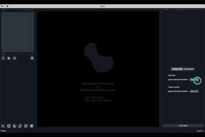
To open the plugin you can click on the "Load spatial single cell" from the Plugins -> napari-sc3d-viewer menu:

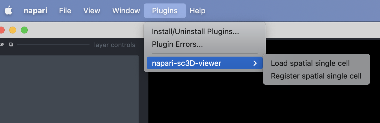
Once opened you should have an interface poping similar to the one showed in the image below (note that it might not be exactly the same depending on the version of the viewer you are using).

Loading and opening a dataset¶

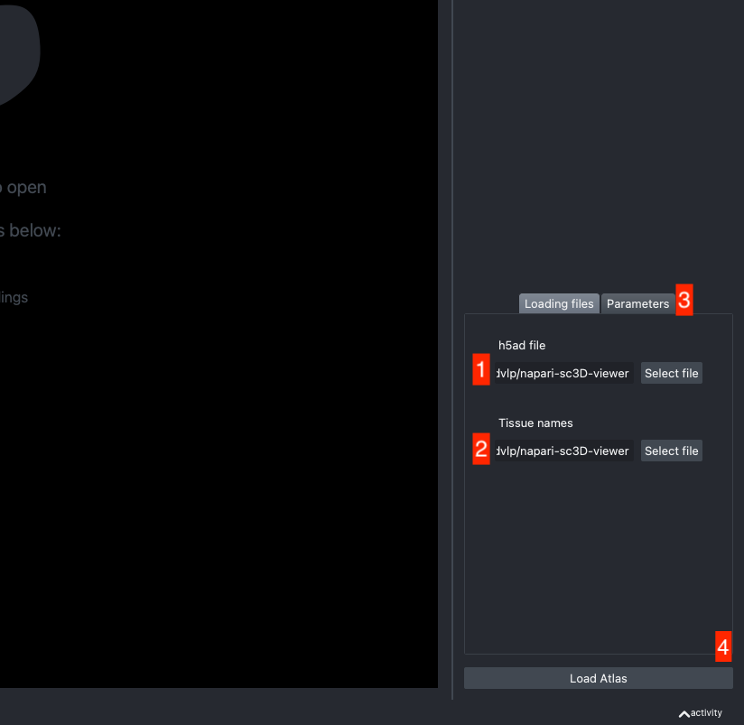
The expected dataset is a scanpy/anndata h5ad file together with an optional json file that maps cluster id numbers to actual tissue/cluster name.

The json file should look like that:

{
    "1": "Endoderm",
    "2": "Heart",
    "10": "Anterior neuroectoderm"
}

If no json file or a wrong json file is given, the original cluster id numbers are used.

The h5ad file should be informed in (1) and the json file in (2).

Let data be your h5ad data structure. To work properly, the viewer is expecting 4 different columns to be present in the h5ad file:

• the cluster id column (by default named 'predicted.id' that can be accessed as data.obs['predicted.id'])
• the 3D position column (by default named 'X_spatial_registered' that can be accessed as data.obsm['X_spatial_registered'])
• the gene names if not already in the column name (by default named 'feature_name' that can be accessed as data.var['feature_name'])
• umap coordinates (by default named 'X_umap' that can be accessed as data.obsm['X_umap'])

If the default column names are not consistent with your dataset, they can be changed in the tab Parameters (3) next to the tab Loading files

Once all the data paths and fields are correctly informed pressing the Load Atlas button (4) will load the dataset.

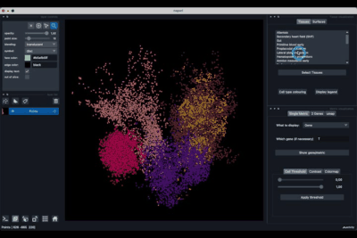
Exploring a dataset¶

Once the dataset is loaded there are few options to explore it.

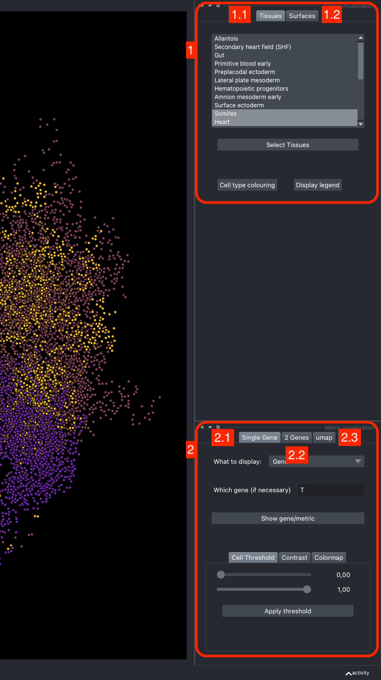
The viewer should look like to the following:

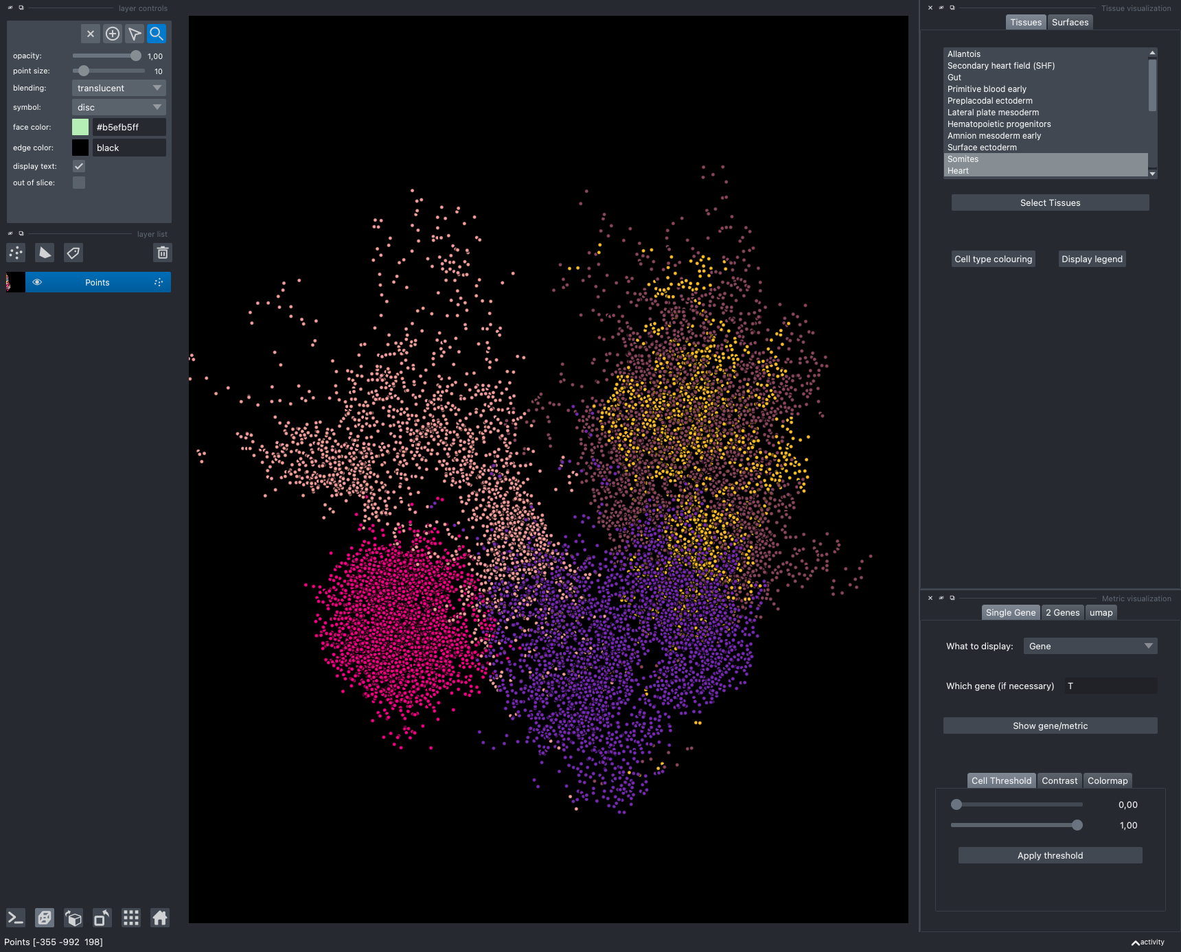
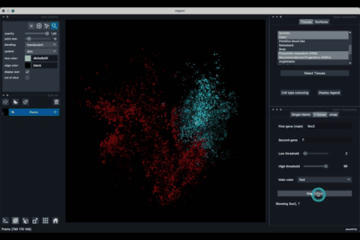
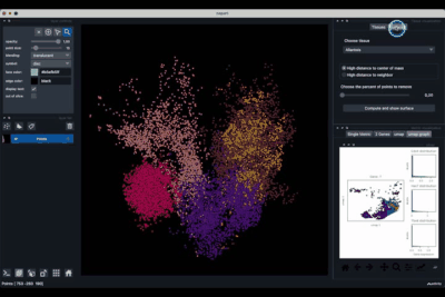
It is divided in two main parts, the Tissue visualisation (1) part and the Metric visualisation (2) one. Both of them are themselves split in two and three tabs respectively. All these tabs allow you to visualise and explore the dataset in different fashions.

The Tissues tab (1.1) allows to select the tissues to display, to show the legend and to colour the cells according to their tissue types.

The Surfaces tab (1.2) allows to construct coarse surfaces of tissues and to display them.

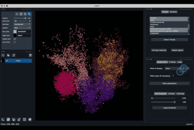
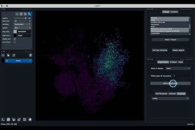
The Single metric tab (2.1) allows to display a metric, whether it is a gene intensity or a numerical metric that is embedded in the visualised dataset. This tab also allows to threshold cells according to the viewed metric, to change the contrast and the colour map.

The 2 Genes (2.2) tab allows to display gene coexpression.

The umap tab (2.3) allows to display the umap of the selected cells and to manually select subcategories of cells to be displayed.

Explanatory "videos"¶

The plugin is meant to be easy to use. That means that you should be able to play with it and figure things out by yourself.

That being said, it is not always that easy. You can find below a series of videos showing how to perform some of the main features.

Loading data¶

Selecting tissues¶

Displaying one gene¶

Displaying two genes co-expression¶

Playing with the umap¶

Computing and processing the surface¶

Contributing¶

Contributions are very welcome. Tests can be run with tox, please ensure the coverage at least stays the same before you submit a pull request.

License¶

Distributed under the terms of the MIT license, "napari-sc3D-viewer" is free and open source software

Issues¶

If you encounter any problems, please file an issue along with a detailed description.